
Efforts to develop indices that mark the bikeability of cities have been the focus of past research. Examples can be found here, here, here, and here.
Bikeability: The term bikeability refers to the level of interaction between factors of the built and natural environments associated with the demand for cycling including infrastructure, slope, land use (destinations), and connectivity. This definition was derived from this study.
This project will map the bikeability of each street link in the city of San Francisco, CA.
The next section briefly describes previous research I modeled this work after. Then the data sources are highlighted in section 2. The methods used in this study are described in section 3, followed by the results in section 4.
1. Vancouver Methodology
This research was modeled after work found here, and is briefly described below.
Winters et al. sought to design a bikeability index that identifies areas more and less suitable for cycling based on commonly available data of ground conditions. The researchers developed methods to measure bikeability across a continuous surface of a 10m-squared grid using a composite index in the Vancouver metro area. The composite bikeability index included bike lane density, bike route separation information, connectivity of bicycle-friendly streets, land use (destinations), and topography. Each factor was partitioned into deciles and subsequently aggregated through the function described below.
Bikeability = (B1 * bicycle route density) + (B2 * bicycle route separation) + (B3 * connectivity of bicycle-friendly streets) + (B4 * topography) + (B5 * destination density)
Where B1 – B5 are the weights allocated to each factor. The study determined the weighting scheme from an opinion survey in the area. The results from the opinion survey suggested where bicycle facility separation data are not available, the overall weighting scheme should double the weight of the bike lane density factor (i.e. B1 = 2, B3 – B5 = 1). However, if bike route density and bike separation data are available, the overall weighting scheme should be balanced (i.e. B1 – B5 = 1).
I won’t go into why these factors were chosen, but if you want information on the importance of connectivity you can see here, here, here, or here. If you want information on the importance of slope, see here, here, here, and here. More information on the importance of land use can be found here, and here. The importance of bike facilities can be read about here, here, here, here, here, here, here, here, here, and here.
The figure below highlights the results from the Vancouver Metro area study.

We can see that the City of Vancouver has a high level of bikeability relative to other parts of the metro area. There are corridors with high levels of bikeability outside the city center. Other patches of high bikeability include east and south-east of the city center, as well as south of the city center. The northern border, as well as the eastern part of the metro area, show low levels of bikeability.
2. Data
This current project leverages a large amount of data from governmental and open sources. Data were prepared and analyzed in QGIS and R. QGIS methods are described below and the full R source code can be found on my GitHub page here. If you’re interested in learning more about the software, you can review the documentation for QGIS here and R here.
- Road links were extracted from OSM using Mapzen’s Metro Extracts.
- Land use and bike lanes were retrieved from OSM, using OSM turbo overpass
- Topographical (slope) data was retrieved from US Dept. of Interior
3. Methods
The GIS methods used to quantify the four factors for each road link are described below. Unlike in the Vancouver study, bike separation data were not available for this current project. Also, this project quantified bikeability at the road link level. Quantifying bikeability at the road link level required less computational power and was therefore much faster/easier to carry out.
Slope – the mean slope was calculated for each road link by importing road link and topographical data into QGIS. A 10meter buffer was created for each road link using the buffer tool. The zonal statistics tool was used to quantify the mean slope for each polygon. Finally, the polygons were joined to the original road links using edge ids.
Bike Lane Density – Bike lane and road link data were imported. The QChainage tool was used to create a poly point layer with a point for every meter of a bike lane. The buffer tool and points in polygon tool were used to count the total meterage of bike lanes surrounding 400 meters of each road link. Values were then joined to the original road link layer by id, and divided by length.
Land Use – Land use and road link data were imported. The points in polygon tool was utilized to count the number of destination points within 400 meters of each road link. Values were then joined to the original road link layer by id, and divided by length.
Connectivity Density of Bike-Friendly Roads – Minor roads were extracted from the road link data. The line intersection tool was used to create a point file of each minor road intersection. The buffer and points in polygon tools were used to count the number of points around each road link in San Francisco. Values were then joined to the original road link layer by id and divided by length.
Notes on Destinations – the following tags were used to extract data from OSM using OSM turbo overpass using the following tags.
- Shop
- amenity = university
- amenity = college
- amenity = school
- amenity = restaurant
- amenity = cafe
- amenity = pub
- amenity = bar
- leisure = park
These sites were chosen based on research on cycling destination from this work by Wu and Rybarczyk, 2010.
Notes on connectivity. Bike friendly roads were considered roads not tagged as motorways, motorway links, and primary roads. This method was modeled after this work by Sun, et al.
R Process
Once each factor was quantified at the road link level, the layer was imported into R as a .dbf file, where it was possible to quantify the composite bikeability index values. If you are familiar with R, you can review the code here.
Each factor for all roads was scored between 1 and 10, where 1 represents least bikeable and 10 represents the most bikeable environment. Once each of the four factors was classified, the bikeability score for each road link was generated using the following function:
Bikeability = (B1 * bicycle route density) + (B2 * connectivity of bicycle-friendly streets) + (B3 * topography) + (B4 * destination density)
Where B1 = 2, and B2 – B4 = 1. Bikeability scores ranged from a low of 5 and a high of 50.
After the bikeability score for each road link was generated, the file was exported as a .csv file from R. This file was subsequently imported into QGIS and joined to the original road link layer.
4. Results
Figure 2 below was generated to visualize the bikeability of San Francisco using the methods described above.

The results of this study indicate high levels of bikeability in the northeast corner of the peninsula (South of Market the Financial District, Lower Haight, and North Beach). The corridors around Visitacion Valley and Haight-Ashbury have developed into bikeable areas. Other positive pockets exist in the areas around San Fransisco area including Parkmerced and the City College of San Francisco.
These areas with a high level of bikeability could be places where social programming, infrastructure projects, policy, and land use tactics may be most effective if they have not already been established. Studies show that safe infrastructure is a driving factor in bicycle use, but a multilateral approach is considered appropriate for the large-scale model shift. These areas may also be places with the lowest level of social risk in terms of capital investments in cycling, as they are areas with the highest level of association with factors important for bicycle use. People in these areas may be more receptive to investments, but more research is needed to validate this idea.
Areas of low levels of bikeability are highlighted in the map by bluer links, including the Sunset District, Lower Pacific Heights, and Excelsior. These areas have rates of factors not associated with cycling. However, as we’ve seen, some cohorts of cyclists prefer opposite values than those used in this study, including Strava users’ preference for steep slopes in some areas.
Feel free to chime in and add your thoughts. And please contact me here if you have any questions.
Keep riding.

that rocks. pagetraffic.com
LikeLike