
This blog post should really be called, How to Measure Centrality Among Bikeshare Trips Using pgRouting and What It Means. I decided against that because, well, the title is already long enough!
In this post, I explore the idea of using pgRouting as a platform to measure trip centrality. I will define centrality, and the steps I took to measure it in a group of bike-share trips that took place in Washington, DC in August of 2019.
Here are the general steps I took to explore this idea:
- Downloaded the relevant data for the tasks, which included:
- An Open Street Map road network of Washington DC from Geofabirk,
- Bikeshare trip data from Capital Bikeshare.
- Built a routable road network using osm2pgrouting
- Constructed an origin-destination table from the station information to feed into pgRouting.
- Defined routing script to measure centrality
- Summarized and visualized the results.
Intro
Lately, I’ve been exploring the routing platform, pgRouting. pgRouting is a great routing engine for tasks like calculating the shortest distance between points, mapping travelsheds, and solving the traveling salesman problem. The beauty of pgRouting is that it’s an extension to PostgreSQL + PostGIS and therefore allows the same kind of relational functionality that makes the SQL family so powerful when executing routing queries.
I’ve talked about how to route bike-share trips in other environments, including R using stplanr, but in this post, I discuss how I built a network and routed 1500 Capital Bikeshare trips from August 2019.
Centrality
Centrality is an extension of graph theory that seeks to measure the importance of different parts of a network. In this case, centrality will be a measure of road segment popularity. We’ll measure this by the number of times a group of trips are passed through a specific segment using a routing algorithm. There are plenty of fancy ways to configure your routing algorithm, but in this case, I used Dijkstra’s short path on a prioritized network (which is a little fancy, I guess, right?).
If you’d like to read more about centrality, here are several papers:
- Trip Centrality: walking on a temporal multiplex with non-instantaneous link travel time
- The role of travel demand and network centrality on the connectivity and resilience of an urban street system
- Centrality and Connectivity in Public Transport Networks and their Significance for Transport Sustainability in Cities
Step 1. Download the Data
If you’re not familiar with Open Street Map, I encourage you to read about it, the foundation, as well as the associated community. In short, it’s a map of the world created and maintained by volunteers. The world map is comprised of spatial vector data and organized by a key:tag system. All of the vector data is available under the Open Data Commons Open Database License.
There are several sources of OSM data, including:
I generally use openstreetmap.org to explore and locate tags, Turbo Overpass to download discrete data (like a specific trail), and GEOFABRIK to extract batch files.
OSM Network
For this application, I downloaded the district-of-columbia-latest.osm.bz file from GEOFABIRK without much exploration. osm2pgrouting can’t read compressed .bz files, but it can read decompressed .osm files, so I used this line of code after navigating to the correct subfolder to decompress .osm for the next step.
bzcat ./osm_data/district-of-columbia-latest.osm.bz2 > ./dc_osm_data.osm
Bike-Share Trip Data
As for the raw bike-share data, I used the raw data from the Capital Bikeshare (CaBi) program. Since the raw trip data doesn’t include origin lat/longs, I also needed station location to join the trip origin. If you’re fancy, you could probably download the json file from online, but I decided to shoot over to the DC open data portal for the station point data. Quick and easy.
Step 2. Building a Routable Network
osm2pgrouting is a very useful tool for building a routable network from OSM data into a PostgreSQL database for pgRouting. osm2pgrouting was designed as another open-source platform to deal with the problems of building a routable network from OSM data using the pgRouting native function, pg_createTopology. The Wiki page for pgRouting says you should assume OSM data is poorly noded, and without osm2pgrouting, suggest you run some additional commands before executing your routing function. I’ve had success creating a half-decent routable OSM network using pgr_nodeNetwork on the street network that results from pg_createtolopogy and subsequently analyzing and cleaning the network. However, osm2pgrouting is so easy once you get the hang of it. One caveat is that osm2pgrouting can struggle with large datasets (such as the entire road network of California). There’s another platform that might be able to handle large datasets that isn’t open source called osm2po. If anyone has experience with this or another platform in handling large datasets, I’d be happy to discuss (OSRM anyone?).
Osm2pgrouing utilizes a configuration file to set network parameters, which is another way to say that you can define the extents and prioritizes your network. For example, you can build a network that omits motorways, which is what I did for this task. The source for osm2pgrouting offers several configurations files to start with on your routing journey.
After I had the decompressed osm file and my servers setup, I ran the following to create my ways and points tables.
osm2pgrouting -f ./dc_osm_data.osm -h localhost -U postgres -d routing --schema dc_routing --prefix dc_b_ -p 5432 -W user --conf=./GitHub/Transportation_Planning/SQL/routing_in_dc/bike_config.xml
Notice I established a prefix on the data to help me organize the information.
The outputs of this included,
- Routable network (ways)
- Vertices table, includes the suffix ‘vertices_pgr’ to your ways table.
Step 3. Construct Origin-Destination Table
To route with pgrouting you need to define your start and end nodes. I used the following script to update my station locations with the nearest start and end node from the vertices table defined in step 2.
CREATE TABLE dc_routing.cabi_stations_updated AS (
  SELECT
    bsst.*,
    vrtx.id as vertex,
    vrtx.distance as distance_to_nn
  FROM (select g.*
        FROM dc_routing.cabi_stations g,
            dc_routing.ruff_dc_outline h
        WHERE ST_INTERSECTS(g.geom, h.geom)) as bsst
  CROSS JOIN LATERAL
    (SELECT
      id,
      ST_DISTANCE(bsst.geom, vtx.the_geom) as distance
    FROM (SELECT *
            FROM dc_routing.dc_ways_vertices_pgr g
            WHERE g.cnt > 2) as vtx
  ORDER BY bsst.geom <-> vtx.the_geom
LIMIT 1) as vrtx
);
This script searches for the nearest node within at least three legs to the station location using a cross-lateral join. The cross-lateral join is probably not the best way to handle this due to computation time, but since we’re dealing with such a small dataset, computational time not a problem.
I subsequently joined this station location information onto a new table of trips to house additional information. Notice here is where I define the trip count to route using the LIMIT clause. I could have handled this better, but what the heck, it’s simple right?
DROP TABLE IF EXISTS    dc_routing.cabi_trips_short;
CREATE TABLE            dc_routing.cabi_trips_short AS (
  SELECT
                        id::INT as old_id,
                        "Duration"::FLOAT as duration,
                        "Start date" as start_date,
                        "End date" as end_date,
                        "Start station number"::INT as start_station_id,
                        "Start station" start_station_name,
                        "End station number"::INT as end_station_id,
                        "End station" as end_station_name,
                        "Bike number" as bike_no,
                        "Member type" as member_type,
                        NULL::FLOAT as start_lat,
                        NULL::FLOAT as start_lon,
                        NULL::FLOAT as end_lat,
                        NULL::FLOAT as end_lon,
                        NULL::geometry(point) as start_geom,
                        NULL::geometry(point) as end_geom,
                        NULL::INT as source_point,
                        NULL::INT as target_point
  FROM                  dc_routing."201908-capitalbikeshare-tripdata"
  LIMIT                 1500
);

UPDATE                  dc_routing.cabi_trips_short gg
SET                     start_lat = g.latitude,
                        start_lon = g.longitude,
                        source_point = g.vertex
FROM                    dc_routing.cabi_stations_updated g
WHERE                   gg.start_station_id = cast(g.terminal_n as integer);

UPDATE                  dc_routing.cabi_trips_short gg
SET                     end_lat = g.latitude,
                        end_lon = g.longitude,
                        target_point = g.vertex
FROM                    dc_routing.cabi_stations_updated g
WHERE                   gg.end_station_id = cast(g.terminal_n as integer);

UPDATE                  dc_routing.cabi_trips_short
set start_geom =        ST_SetSRID(ST_MAKEPOINT(start_lon, start_lat), 4326),
end_geom =              ST_SETSRID(ST_MAKEPOINT(end_lon, end_lat), 4326);
After this, I established a cost value on my road segments. This step is required for the routing algorithm to determine the amount of travel along a segment. In this application, I decided to use length as my cost parameter.
UPDATE        dc_routing.dc_ways
SET           cost_f_ft = ST_length(the_geom),
              cost_r_ft = ST_length(the_geom);
Step 4. Defined routing script to measure centrality
Testing my setup
I wanted to test to see if my engine worked and trips were routable, so I wrote a script to infer the shortest path for each trip during the study period. I ended up with routes for each trip. You can see I’ve highlighted trip id 1600 to illustrate the data resulting structure.
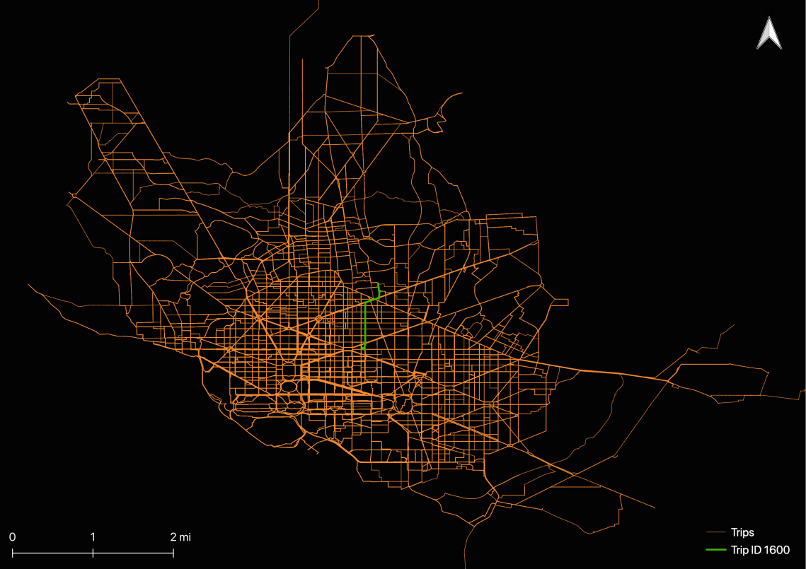
Another possible way to think about these individual lines is an inferred route chosen by the user. I doubt these are very valid. There are a lot of ways we could measure this, such as comparing actual trip lengths/times to inferred trip lengths/times.
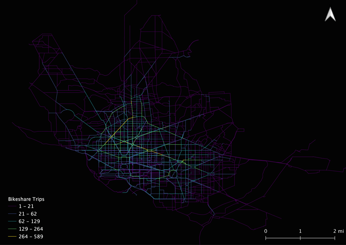
Measuring centrality
The second script that I executed aggregated the geometries by geom ID, rather than bike-share trip ID. In the end, I ended up with a data frame of road segments with a count of trips the routing algorithm sent through each segment. This is a basic way of defining the centrality, and in this case, the segments most often used by the bike-share users during our study period.
Here’re the script I used to generate measures of centrality.
DROP TABLE IF EXISTS dc_routing.trips_centrality;
CREATE TABLE dc_routing.trips_centrality as (
SELECT
  b.gid,
  b.the_geom as geom,
  count(the_geom) as count
FROM
dc_routing.cabi_trips_short gg
  pgr_dijkstra(
      'SELECT
          g.gid as id,
          g.source,
          g.target,
          g.length as cost
          FROM dc_routing.dc_ways g',
               gg.source_point,
               gg.target_point,
               directed := FALSE) j
          JOIN    dc_routing.dc_ways AS b
            ON    j.edge = b.gid
GROUP BY b.gid, b.the_geom, gg.member_type);
Step 5. Visual and summarize
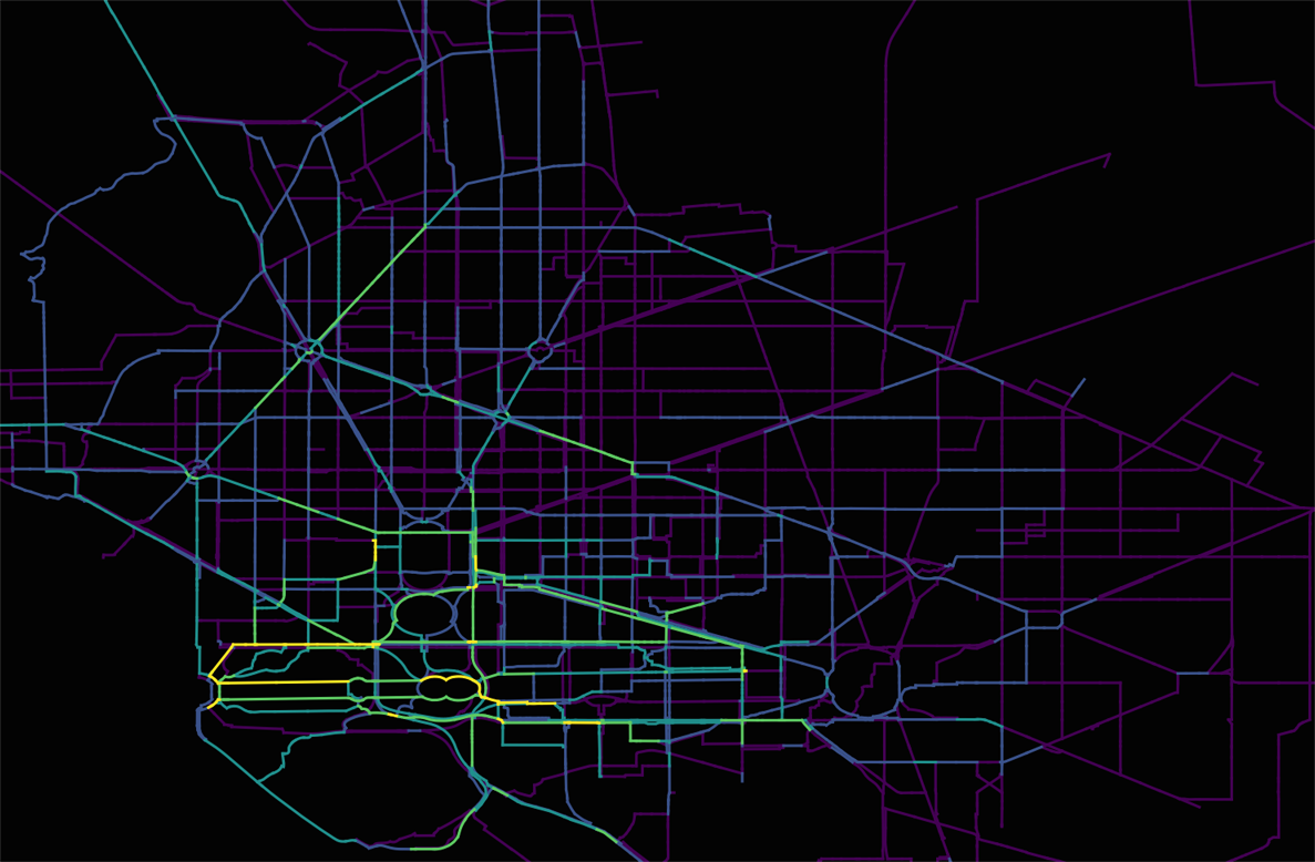
Here are the results from the script above, color gradient over count:
Obviously, this doesn’t accurately reflect reality, but it shines a light on how we can start to think about our bike-share trip data in relation to our road network. Specifically, we can begin to think about how we can answer the difficult question of where do people ride bikes?
Down the line, if we can verify the routing algorithm, then we could start to point to areas on the network to prioritize investments. We can point to road segments where people ride bikes say, “perhaps we should spend money on this location to increase safety and network quality for bicyclists”. Perhaps the argument for building buffered bike lanes, fix potholes, and improving intersections will be easier with this inferred measure of use.
I also took a minute to measure centrality on user types. I measured centrality among members and casual users. The results are surprising.
Centrality of Member Trips
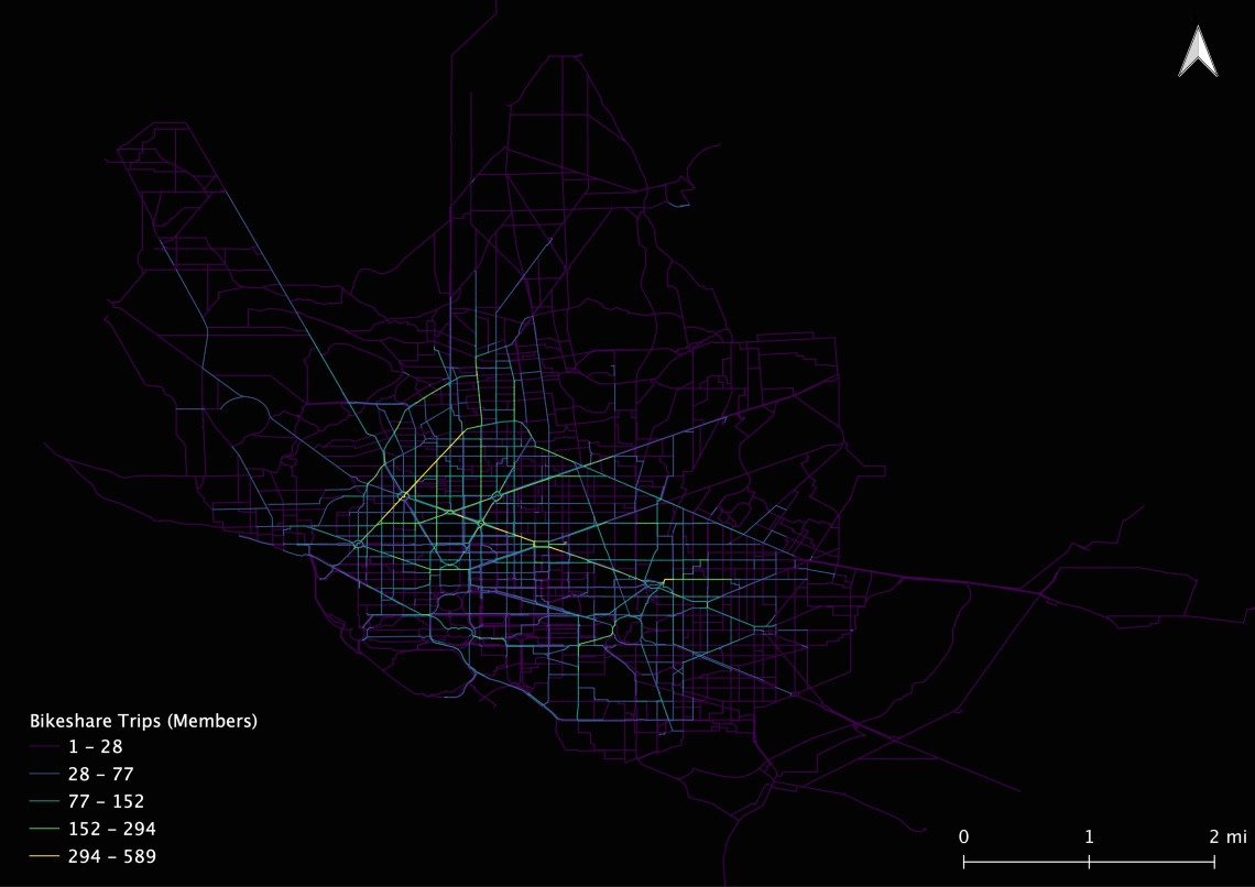
Centrality of Casual Trips

Together these images tell us two things:
- That casual users primarily used bike-share in the southwest of DC near Georgetown and the National Mall (this is not surprising)
- Members primarily rode across the city using major arterials.
I want to point out here that I only routed 1500 trips, which is especially problematic for reviewing these user type maps because I didn’t control for user type distribution. Again, this post is intended for us to explore the idea of centrality on bike-share trip data using pgRouting.
In sum, this would seem like a good starting point to apply this at scale. One problem that needs further discussion is computational time. This task took a while to finish, and would not be appropriate across a large number of trips. I’m currently exploring OSRM to apply the same workflow discussed hear across a large area, using many more trips.
For more information on pgRouting, the manual can be found here:
https://docs.pgrouting.org/latest/en/index.html
Happy routing!

Thanks for possting this
LikeLike